![]() v1.6
v1.6
Streaming Concepts
Flink’s Table API and SQL support are unified APIs for batch and stream processing. This means that Table API and SQL queries have the same semantics regardless whether their input is bounded batch input or unbounded stream input. Because the relational algebra and SQL were originally designed for batch processing, relational queries on unbounded streaming input are not as well understood as relational queries on bounded batch input.
On this page, we explain concepts, practical limitations, and stream-specific configuration parameters of Flink’s relational APIs on streaming data.
- Relational Queries on Data Streams
- Dynamic Tables & Continuous Queries
- Time Attributes
- Query Configuration
Relational Queries on Data Streams
SQL and the relational algebra have not been designed with streaming data in mind. As a consequence, there are few conceptual gaps between relational algebra (and SQL) and stream processing.
| Relational Algebra / SQL | Stream Processing |
|---|---|
| Relations (or tables) are bounded (multi-)sets of tuples. | A stream is an infinite sequences of tuples. |
| A query that is executed on batch data (e.g., a table in a relational database) has access to the complete input data. | A streaming query cannot access all data when is started and has to "wait" for data to be streamed in. |
| A batch query terminates after it produced a fixed sized result. | A streaming query continuously updates its result based on the received records and never completes. |
Despite these differences, processing streams with relational queries and SQL is not impossible. Advanced relational database systems offer a feature called Materialized Views. A materialized view is defined as a SQL query, just like a regular virtual view. In contrast to a virtual view, a materialized view caches the result of the query such that the query does not need to be evaluated when the view is accessed. A common challenge for caching is to prevent a cache from serving outdated results. A materialized view becomes outdated when the base tables of its definition query are modified. Eager View Maintenance is a technique to update materialized views and updates a materialized view as soon as its base tables are updated.
The connection between eager view maintenance and SQL queries on streams becomes obvious if we consider the following:
- A database table is the result of a stream of
INSERT,UPDATE, andDELETEDML statements, often called changelog stream. - A materialized view is defined as a SQL query. In order to update the view, the query is continuously processes the changelog streams of the view’s base relations.
- The materialized view is the result of the streaming SQL query.
With these points in mind, we introduce Flink’s concept of Dynamic Tables in the next section.
Dynamic Tables & Continuous Queries
Dynamic tables are the core concept of Flink’s Table API and SQL support for streaming data. In contrast to the static tables that represent batch data, dynamic table are changing over time. They can be queried like static batch tables. Querying a dynamic table yields a Continuous Query. A continuous query never terminates and produces a dynamic table as result. The query continuously updates its (dynamic) result table to reflect the changes on its input (dynamic) table. Essentially, a continuous query on a dynamic table is very similar to the definition query of a materialized view.
It is important to note that the result of a continuous query is always semantically equivalent to the result of the same query being executed in batch mode on a snapshot of the input tables.
The following figure visualizes the relationship of streams, dynamic tables, and continuous queries:

- A stream is converted into a dynamic table.
- A continuous query is evaluated on the dynamic table yielding a new dynamic table.
- The resulting dynamic table is converted back into a stream.
Note: Dynamic tables are foremost a logical concept. Dynamic tables are not necessarily (fully) materialized during query execution.
In the following, we will explain the concepts of dynamic tables and continuous queries with a stream of click events that have the following schema:
[
  user:  VARCHAR,   // the name of the user
  cTime: TIMESTAMP, // the time when the URL was accessed
  url:   VARCHAR    // the URL that was accessed by the user
]
Defining a Table on a Stream
In order to process a stream with a relational query, it has to be converted into a Table. Conceptually, each record of the stream is interpreted as an INSERT modification on the resulting table. Essentially, we are building a table from an INSERT-only changelog stream.
The following figure visualizes how the stream of click event (left-hand side) is converted into a table (right-hand side). The resulting table is continuously growing as more records of the click stream are inserted.
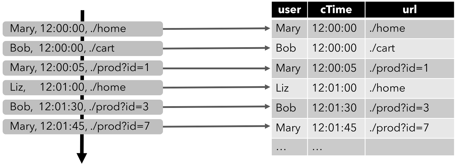
Note: A table which is defined on a stream is internally not materialized.
Continuous Queries
A continuous query is evaluated on a dynamic table and produces a new dynamic table as result. In contrast to a batch query, a continuous query never terminates and updates its result table according to the updates on its input tables. At any point in time, the result of a continuous query is semantically equivalent to the result of the same query being executed in batch mode on a snapshot of the input tables.
In the following we show two example queries on a clicks table that is defined on the stream of click events.
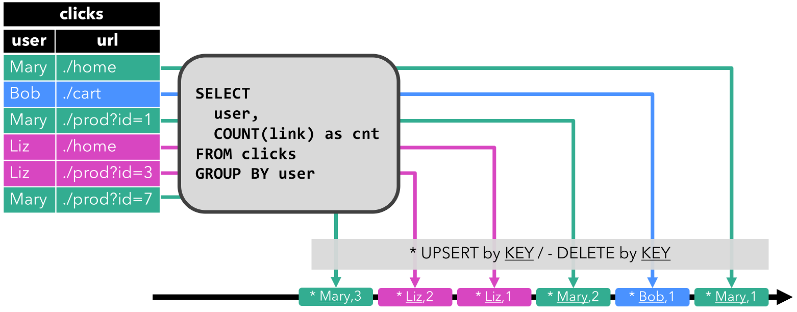
The first query is a simple GROUP-BY COUNT aggregation query. It groups the clicks table on the user field and counts the number of visited URLs. The following figure shows how the query is evaluated over time as the clicks table is updated with additional rows.
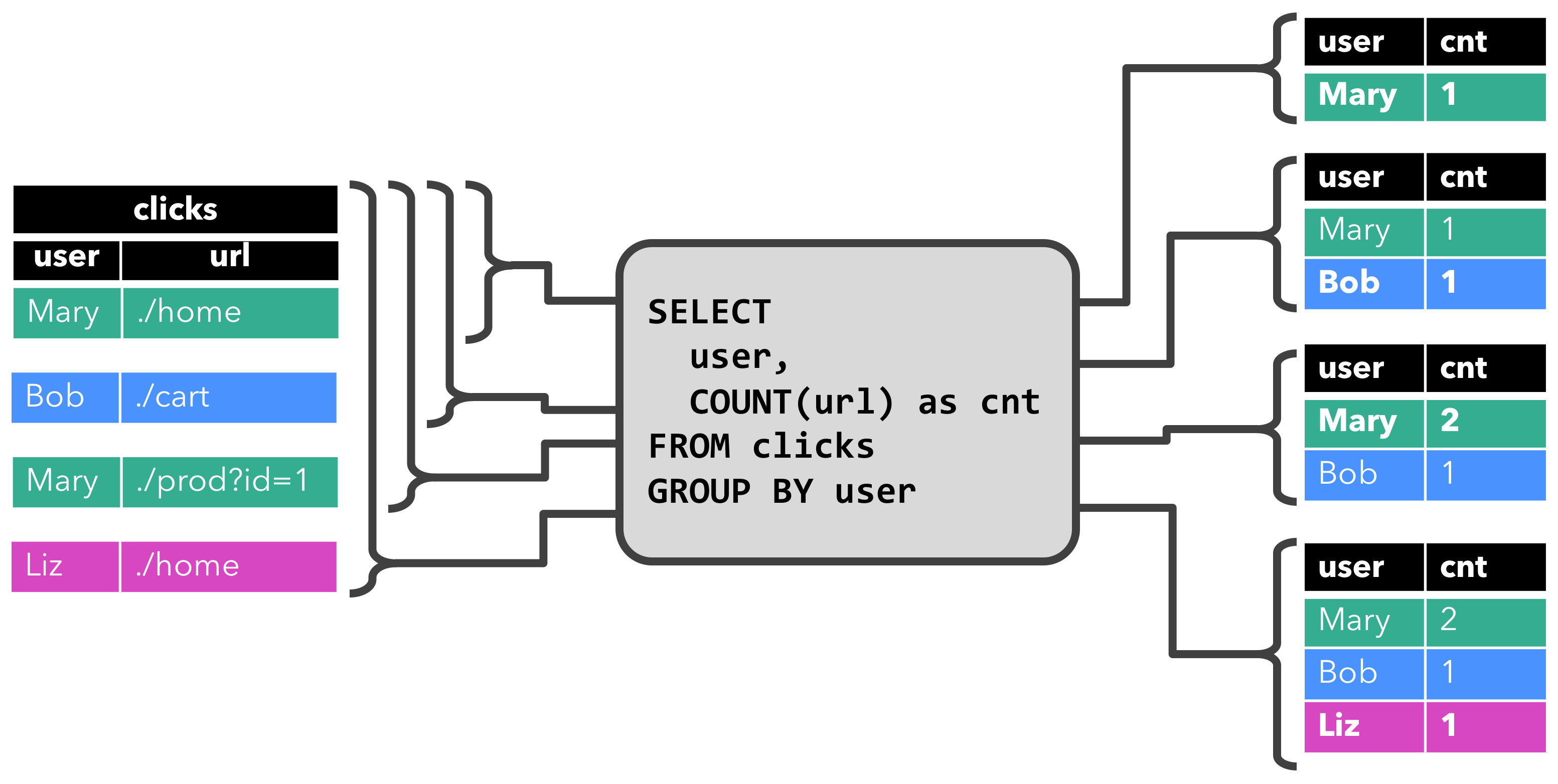
When the query is started, the clicks table (left-hand side) is empty. The query starts to compute the result table, when the first row is inserted into the clicks table. After the first row [Mary, ./home] was inserted, the result table (right-hand side, top) consists of a single row [Mary, 1]. When the second row [Bob, ./cart] is inserted into the clicks table, the query updates the result table and inserts a new row [Bob, 1]. The third row [Mary, ./prod?id=1] yields an update of an already computed result row such that [Mary, 1] is updated to [Mary, 2]. Finally, the query inserts a third row [Liz, 1] into the result table, when the fourth row is appended to the clicks table.
The second query is similar to the first one but groups the clicks table in addition to the user attribute also on an hourly tumbling window before it counts the number of URLs (time-based computations such as windows are based on special time attributes, which are discussed below.). Again, the figure shows the input and output at different points in time to visualize the changing nature of dynamic tables.
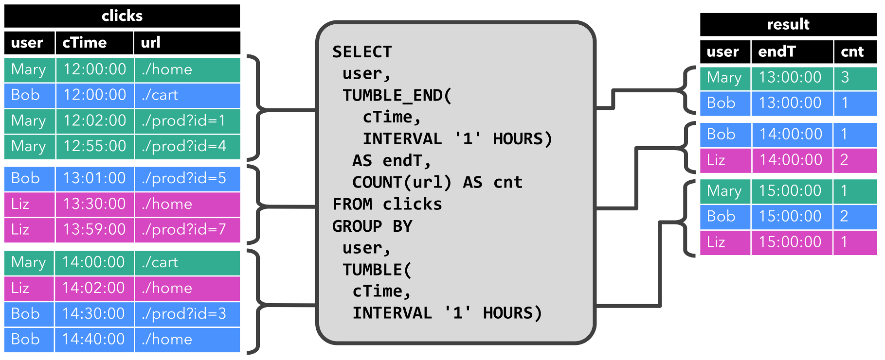
As before, the input table clicks is shown on the left. The query continuously computes results every hour and updates the result table. The clicks table contains four rows with timestamps (cTime) between 12:00:00 and 12:59:59. The query computes two results rows from this input (one for each user) and appends them to the result table. For the next window between 13:00:00 and 13:59:59, the clicks table contains three rows, which results in another two rows being appended to the result table. The result table is updated, as more rows are appended to clicks over time.
Update and Append Queries
Although the two example queries appear to be quite similar (both compute a grouped count aggregate), they differ in one important aspect:
- The first query updates previously emitted results, i.e., the changelog stream that defines the result table contains
INSERTandUPDATEchanges. - The second query only appends to the result table, i.e., the changelog stream of the result table only consists of
INSERTchanges.
Whether a query produces an append-only table or an updated table has some implications:
- Queries that produce update changes usually have to maintain more state (see the following section).
- The conversion of an append-only table into a stream is different from the conversion of an updated table (see the Table to Stream Conversion section).
Query Restrictions
Many, but not all, semantically valid queries can be evaluated as continuous queries on streams. Some queries are too expensive to compute, either due to the size of state that they need to maintain or because computing updates is too expensive.
- State Size: Continuous queries are evaluated on unbounded streams and are often supposed to run for weeks or months. Hence, the total amount of data that a continuous query processes can be very large. Queries that have to update previously emitted results need to maintain all emitted rows in order to be able to update them. For instance, the first example query needs to store the URL count for each user to be able to increase the count and sent out a new result when the input table receives a new row. If only registered users are tracked, the number of counts to maintain might not be too high. However, if non-registered users get a unique user name assigned, the number of counts to maintain would grow over time and might eventually cause the query to fail.
SELECT user, COUNT(url)
FROM clicks
GROUP BY user;- Computing Updates: Some queries require to recompute and update a large fraction of the emitted result rows even if only a single input record is added or updated. Clearly, such queries are not well suited to be executed as continuous queries. An example is the following query which computes for each user a
RANKbased on the time of the last click. As soon as theclickstable receives a new row, thelastActionof the user is updated and a new rank must be computed. However since two rows cannot have the same rank, all lower ranked rows need to be updated as well.
SELECT user, RANK() OVER (ORDER BY lastLogin)
FROM (
  SELECT user, MAX(cTime) AS lastAction FROM clicks GROUP BY user
);
The QueryConfig section discusses parameters to control the execution of continuous queries. Some parameters can be used to trade the size of maintained state for result accuracy.
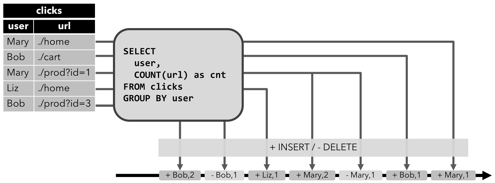
Table to Stream Conversion
A dynamic table can be continuously modified by INSERT, UPDATE, and DELETE changes just like a regular database table. It might be a table with a single row, which is constantly updated, an insert-only table without UPDATE and DELETE modifications, or anything in between.
When converting a dynamic table into a stream or writing it to an external system, these changes need to be encoded. Flink’s Table API and SQL support three ways to encode the changes of a dynamic table:
-
Append-only stream: A dynamic table that is only modified by
INSERTchanges can be converted into a stream by emitting the inserted rows. -
Retract stream: A retract stream is a stream with two types of messages, add messages and retract messages. A dynamic table is converted into an retract stream by encoding an
INSERTchange as add message, aDELETEchange as retract message, and anUPDATEchange as a retract message for the updated (previous) row and an add message for the updating (new) row. The following figure visualizes the conversion of a dynamic table into a retract stream.
- Upsert stream: An upsert stream is a stream with two types of messages, upsert messages and delete message. A dynamic table that is converted into an upsert stream requires a (possibly composite) unique key. A dynamic table with unique key is converted into a dynamic table by encoding
INSERTandUPDATEchanges as upsert message andDELETEchanges as delete message. The stream consuming operator needs to be aware of the unique key attribute in order to apply messages correctly. The main difference to a retract stream is thatUPDATEchanges are encoded with a single message and hence more efficient. The following figure visualizes the conversion of a dynamic table into an upsert stream.
The API to convert a dynamic table into a DataStream is discussed on the Common Concepts page. Please note that only append and retract streams are supported when converting a dynamic table into a DataStream. The TableSink interface to emit a dynamic table to an external system are discussed on the TableSources and TableSinks page.
Time Attributes
Flink is able to process streaming data based on different notions of time.
- Processing time refers to the system time of the machine (also known as “wall-clock time”) that is executing the respective operation.
- Event time refers to the processing of streaming data based on timestamps which are attached to each row. The timestamps can encode when an event happened.
- Ingestion time is the time that events enter Flink; internally, it is treated similarly to event time.
For more information about time handling in Flink, see the introduction about Event Time and Watermarks.
Table programs require that the corresponding time characteristic has been specified for the streaming environment:
final StreamExecutionEnvironment env = StreamExecutionEnvironment.getExecutionEnvironment();

env.setStreamTimeCharacteristic(TimeCharacteristic.ProcessingTime); // default

// alternatively:
// env.setStreamTimeCharacteristic(TimeCharacteristic.IngestionTime);
// env.setStreamTimeCharacteristic(TimeCharacteristic.EventTime);
val env = StreamExecutionEnvironment.getExecutionEnvironment
env.setStreamTimeCharacteristic(TimeCharacteristic.ProcessingTime) // default
// alternatively:
// env.setStreamTimeCharacteristic(TimeCharacteristic.IngestionTime)
// env.setStreamTimeCharacteristic(TimeCharacteristic.EventTime)Time-based operations such as windows in both the Table API and SQL require information about the notion of time and its origin. Therefore, tables can offer logical time attributes for indicating time and accessing corresponding timestamps in table programs.
Time attributes can be part of every table schema. They are defined when creating a table from a DataStream or are pre-defined when using a TableSource. Once a time attribute has been defined at the beginning, it can be referenced as a field and can used in time-based operations.
As long as a time attribute is not modified and is simply forwarded from one part of the query to another, it remains a valid time attribute. Time attributes behave like regular timestamps and can be accessed for calculations. If a time attribute is used in a calculation, it will be materialized and becomes a regular timestamp. Regular timestamps do not cooperate with Flink’s time and watermarking system and thus can not be used for time-based operations anymore.
Processing time
Processing time allows a table program to produce results based on the time of the local machine. It is the simplest notion of time but does not provide determinism. It neither requires timestamp extraction nor watermark generation.
There are two ways to define a processing time attribute.
During DataStream-to-Table Conversion
The processing time attribute is defined with the .proctime property during schema definition. The time attribute must only extend the physical schema by an additional logical field. Thus, it can only be defined at the end of the schema definition.
DataStream<Tuple2<String, String>> stream = ...;

// declare an additional logical field as a processing time attribute
Table table = tEnv.fromDataStream(stream, "Username, Data, UserActionTime.proctime");

WindowedTable windowedTable = table.window(Tumble.over("10.minutes").on("UserActionTime").as("userActionWindow"));
val stream: DataStream[(String, String)] = ...
// declare an additional logical field as a processing time attribute
val table = tEnv.fromDataStream(stream, 'UserActionTimestamp, 'Username, 'Data, 'UserActionTime.proctime)
val windowedTable = table.window(Tumble over 10.minutes on 'UserActionTime as 'userActionWindow)Using a TableSource
The processing time attribute is defined by a TableSource that implements the DefinedProctimeAttribute interface. The logical time attribute is appended to the physical schema defined by the return type of the TableSource.
// define a table source with a processing attribute
public class UserActionSource implements StreamTableSource<Row>, DefinedProctimeAttribute {

	@Override
	public TypeInformation<Row> getReturnType() {
		String[] names = new String[] {"Username" , "Data"};
		TypeInformation[] types = new TypeInformation[] {Types.STRING(), Types.STRING()};
		return Types.ROW(names, types);
	}

	@Override
	public DataStream<Row> getDataStream(StreamExecutionEnvironment execEnv) {
		// create stream
		DataStream<Row> stream = ...;
		return stream;
	}

	@Override
	public String getProctimeAttribute() {
		// field with this name will be appended as a third field
		return "UserActionTime";
	}
}

// register table source
tEnv.registerTableSource("UserActions", new UserActionSource());

WindowedTable windowedTable = tEnv
	.scan("UserActions")
	.window(Tumble.over("10.minutes").on("UserActionTime").as("userActionWindow"));
// define a table source with a processing attribute
class UserActionSource extends StreamTableSource[Row] with DefinedProctimeAttribute {
override def getReturnType = {
val names = Array[String]("Username" , "Data")
val types = Array[TypeInformation[_]](Types.STRING, Types.STRING)
Types.ROW(names, types)
}
override def getDataStream(execEnv: StreamExecutionEnvironment): DataStream[Row] = {
// create stream
val stream = ...
stream
}
override def getProctimeAttribute = {
// field with this name will be appended as a third field
"UserActionTime"
}
}
// register table source
tEnv.registerTableSource("UserActions", new UserActionSource)
val windowedTable = tEnv
.scan("UserActions")
.window(Tumble over 10.minutes on 'UserActionTime as 'userActionWindow)Event time
Event time allows a table program to produce results based on the time that is contained in every record. This allows for consistent results even in case of out-of-order events or late events. It also ensures replayable results of the table program when reading records from persistent storage.
Additionally, event time allows for unified syntax for table programs in both batch and streaming environments. A time attribute in a streaming environment can be a regular field of a record in a batch environment.
In order to handle out-of-order events and distinguish between on-time and late events in streaming, Flink needs to extract timestamps from events and make some kind of progress in time (so-called watermarks).
An event time attribute can be defined either during DataStream-to-Table conversion or by using a TableSource.
During DataStream-to-Table Conversion
The event time attribute is defined with the .rowtime property during schema definition. Timestamps and watermarks must have been assigned in the DataStream that is converted.
There are two ways of defining the time attribute when converting a DataStream into a Table. Depending on whether the specified .rowtime field name exists in the schema of the DataStream or not, the timestamp field is either
- appended as a new field to the schema or
- replaces an existing field.
In either case the event time timestamp field will hold the value of the DataStream event time timestamp.
// Option 1:

// extract timestamp and assign watermarks based on knowledge of the stream
DataStream<Tuple2<String, String>> stream = inputStream.assignTimestampsAndWatermarks(...);

// declare an additional logical field as an event time attribute
Table table = tEnv.fromDataStream(stream, "Username, Data, UserActionTime.rowtime");


// Option 2:

// extract timestamp from first field, and assign watermarks based on knowledge of the stream
DataStream<Tuple3<Long, String, String>> stream = inputStream.assignTimestampsAndWatermarks(...);

// the first field has been used for timestamp extraction, and is no longer necessary
// replace first field with a logical event time attribute
Table table = tEnv.fromDataStream(stream, "UserActionTime.rowtime, Username, Data");

// Usage:

WindowedTable windowedTable = table.window(Tumble.over("10.minutes").on("UserActionTime").as("userActionWindow"));
// Option 1:
// extract timestamp and assign watermarks based on knowledge of the stream
val stream: DataStream[(String, String)] = inputStream.assignTimestampsAndWatermarks(...)
// declare an additional logical field as an event time attribute
val table = tEnv.fromDataStream(stream, 'Username, 'Data, 'UserActionTime.rowtime)
// Option 2:
// extract timestamp from first field, and assign watermarks based on knowledge of the stream
val stream: DataStream[(Long, String, String)] = inputStream.assignTimestampsAndWatermarks(...)
// the first field has been used for timestamp extraction, and is no longer necessary
// replace first field with a logical event time attribute
val table = tEnv.fromDataStream(stream, 'UserActionTime.rowtime, 'Username, 'Data)
// Usage:
val windowedTable = table.window(Tumble over 10.minutes on 'UserActionTime as 'userActionWindow)Using a TableSource
The event time attribute is defined by a TableSource that implements the DefinedRowtimeAttributes interface. The getRowtimeAttributeDescriptors() method returns a list of RowtimeAttributeDescriptor for describing the final name of a time attribute, a timestamp extractor to derive the values of the attribute, and the watermark strategy associated with the attribute.
Please make sure that the DataStream returned by the getDataStream() method is aligned with the defined time attribute.
The timestamps of the DataStream (the ones which are assigned by a TimestampAssigner) are only considered if a StreamRecordTimestamp timestamp extractor is defined.
Watermarks of a DataStream are only preserved if a PreserveWatermarks watermark strategy is defined.
Otherwise, only the values of the TableSource’s rowtime attribute are relevant.
// define a table source with a rowtime attribute
public class UserActionSource implements StreamTableSource<Row>, DefinedRowtimeAttributes {

	@Override
	public TypeInformation<Row> getReturnType() {
		String[] names = new String[] {"Username", "Data", "UserActionTime"};
		TypeInformation[] types =
			new TypeInformation[] {Types.STRING(), Types.STRING(), Types.LONG()};
		return Types.ROW(names, types);
	}

	@Override
	public DataStream<Row> getDataStream(StreamExecutionEnvironment execEnv) {
		// create stream
		// ...
		// assign watermarks based on the "UserActionTime" attribute
		DataStream<Row> stream = inputStream.assignTimestampsAndWatermarks(...);
		return stream;
	}

	@Override
	public List<RowtimeAttributeDescriptor> getRowtimeAttributeDescriptors() {
		// Mark the "UserActionTime" attribute as event-time attribute.
		// We create one attribute descriptor of "UserActionTime".
		RowtimeAttributeDescriptor rowtimeAttrDescr = new RowtimeAttributeDescriptor(
			"UserActionTime",
			new ExistingField("UserActionTime"),
			new AscendingTimestamps());
		List<RowtimeAttributeDescriptor> listRowtimeAttrDescr = Collections.singletonList(rowtimeAttrDescr);
		return listRowtimeAttrDescr;
	}
}

// register the table source
tEnv.registerTableSource("UserActions", new UserActionSource());

WindowedTable windowedTable = tEnv
	.scan("UserActions")
	.window(Tumble.over("10.minutes").on("UserActionTime").as("userActionWindow"));
// define a table source with a rowtime attribute
class UserActionSource extends StreamTableSource[Row] with DefinedRowtimeAttributes {
override def getReturnType = {
val names = Array[String]("Username" , "Data", "UserActionTime")
val types = Array[TypeInformation[_]](Types.STRING, Types.STRING, Types.LONG)
Types.ROW(names, types)
}
override def getDataStream(execEnv: StreamExecutionEnvironment): DataStream[Row] = {
// create stream
// ...
// assign watermarks based on the "UserActionTime" attribute
val stream = inputStream.assignTimestampsAndWatermarks(...)
stream
}
override def getRowtimeAttributeDescriptors: util.List[RowtimeAttributeDescriptor] = {
// Mark the "UserActionTime" attribute as event-time attribute.
// We create one attribute descriptor of "UserActionTime".
val rowtimeAttrDescr = new RowtimeAttributeDescriptor(
"UserActionTime",
new ExistingField("UserActionTime"),
new AscendingTimestamps)
val listRowtimeAttrDescr = Collections.singletonList(rowtimeAttrDescr)
listRowtimeAttrDescr
}
}
// register the table source
tEnv.registerTableSource("UserActions", new UserActionSource)
val windowedTable = tEnv
.scan("UserActions")
.window(Tumble over 10.minutes on 'UserActionTime as 'userActionWindow)Query Configuration
Table API and SQL queries have the same semantics regardless whether their input is bounded batch input or unbounded stream input. In many cases, continuous queries on streaming input are capable of computing accurate results that are identical to offline computed results. However, this is not possible in general case because continuous queries have to restrict the size of the state they are maintaining in order to avoid to run out of storage and to be able to process unbounded streaming data over a long period of time. As a result, a continuous query might only be able to provide approximated results depending on the characteristics of the input data and the query itself.
Flink’s Table API and SQL interface provide parameters to tune the accuracy and resource consumption of continuous queries. The parameters are specified via a QueryConfig object. The QueryConfig can be obtained from the TableEnvironment and is passed back when a Table is translated, i.e., when it is transformed into a DataStream or emitted via a TableSink.
StreamExecutionEnvironment env = StreamExecutionEnvironment.getExecutionEnvironment();
StreamTableEnvironment tableEnv = TableEnvironment.getTableEnvironment(env);

// obtain query configuration from TableEnvironment
StreamQueryConfig qConfig = tableEnv.queryConfig();
// set query parameters
qConfig.withIdleStateRetentionTime(Time.hours(12), Time.hours(24));

// define query
Table result = ...

// create TableSink
TableSink<Row> sink = ...

// emit result Table via a TableSink
result.writeToSink(sink, qConfig);

// convert result Table into a DataStream<Row>
DataStream<Row> stream = tableEnv.toAppendStream(result, Row.class, qConfig);
val env = StreamExecutionEnvironment.getExecutionEnvironment
val tableEnv = TableEnvironment.getTableEnvironment(env)
// obtain query configuration from TableEnvironment
val qConfig: StreamQueryConfig = tableEnv.queryConfig
// set query parameters
qConfig.withIdleStateRetentionTime(Time.hours(12), Time.hours(24))
// define query
val result: Table = ???
// create TableSink
val sink: TableSink[Row] = ???
// emit result Table via a TableSink
result.writeToSink(sink, qConfig)
// convert result Table into a DataStream[Row]
val stream: DataStream[Row] = result.toAppendStream[Row](qConfig)In the following we describe the parameters of the QueryConfig and how they affect the accuracy and resource consumption of a query.
Idle State Retention Time
Many queries aggregate or join records on one or more key attributes. When such a query is executed on a stream, the continuous query needs to collect records or maintain partial results per key. If the key domain of the input stream is evolving, i.e., the active key values are changing over time, the continuous query accumulates more and more state as more and more distinct keys are observed. However, often keys become inactive after some time and their corresponding state becomes stale and useless.
For example the following query computes the number of clicks per session.
SELECT sessionId, COUNT(*) FROM clicks GROUP BY sessionId;The sessionId attribute is used as a grouping key and the continuous query maintains a count for each sessionId it observes. The sessionId attribute is evolving over time and sessionId values are only active until the session ends, i.e., for a limited period of time. However, the continuous query cannot know about this property of sessionId and expects that every sessionId value can occur at any point of time. It maintains a count for each observed sessionId value. Consequently, the total state size of the query is continuously growing as more and more sessionId values are observed.
The Idle State Retention Time parameters define for how long the state of a key is retained without being updated before it is removed. For the previous example query, the count of a sessionId would be removed as soon as it has not been updated for the configured period of time.
By removing the state of a key, the continuous query completely forgets that it has seen this key before. If a record with a key, whose state has been removed before, is processed, the record will be treated as if it was the first record with the respective key. For the example above this means that the count of a sessionId would start again at 0.
There are two parameters to configure the idle state retention time:
- The minimum idle state retention time defines how long the state of an inactive key is at least kept before it is removed.
- The maximum idle state retention time defines how long the state of an inactive key is at most kept before it is removed.
The parameters are specified as follows:
StreamQueryConfig qConfig = ...

// set idle state retention time: min = 12 hours, max = 24 hours
qConfig.withIdleStateRetentionTime(Time.hours(12), Time.hours(24));
val qConfig: StreamQueryConfig = ???
// set idle state retention time: min = 12 hours, max = 24 hours
qConfig.withIdleStateRetentionTime(Time.hours(12), Time.hours(24))Cleaning up state requires additional bookkeeping which becomes less expensive for larger differences of minTime and maxTime. The difference between minTime and maxTime must be at least 5 minutes.